About Me!

This blog is about my musings and thoughts. I hope you find it useful, at most, and entertaining, at least.
Other Pages
Presence Elsewhere
Calculating Service Area, Part 2: Defining the Walkshed
Date: 2019-01-10
Tags: postgis pg-routing postgres gis gtfs transit census
In Part 1 we talked about the project and got some of the tools and data we need to start. A quick reminder of our motivation: to figure out the percentage area and population the county transit agency serves by using a "walkshed". A walkshed is the distance from a busstop, along the road for a certain distance. We'll talk more later in this article why it's important to be along the road. Once we have a walkshed, we'll use census data to compute the statistics we're interested in.
Parts
- Part 1: Introduction and Setup
- Part 2: Defining the Walkshed
- Part 3: Demographics
- Part 4: Next Steps
Defining Distance
At this point, we have enough data to start playing around with. However, if
we examine a random road from the ways table in QGIS, we'll notice that its
length is something like "0.0007016736064598".
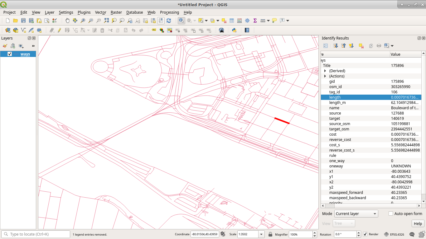
You might be thinking that those are some funny units. You wouldn't be far off; they're units of degrees. They're not insensible units, especially given that our geographic data has a project on WGS 84 (EPSG 4326) (GPS Coördinates, which are in-fact in degrees), but they're not very useful for what we're trying to do.
Reprojection
In order to deal with more useful units, feet, we need to reproject, convert it into a new coordinate system, the data. (I discuss projections a little more at Projections and Why They're Important.) I'm going to choose the Pennsylvania South State Plane (EPSG 3365), which is designed to provide an accurate plane in linear units (3365 is feet, 3364 is in meters) in the southern portion of Pennsylvania. Being able to work in linear units is significantly easier, and significantly more accurate, when doing analysis like this that is based on requirements in linear units.
To convert the geometries we currently have, we'll copy the tables (to retain the source data) and then reproject those in-place. The reason we need to reproject the stops and blocks is that the geographic operations like selecting within a certain distance work best when everything is in the same projection. (QGIS would display everything correctly, but PostGIS doesn't like doing spatial operations over different projections.) I also took this oppurtunity to filter the block data to just Allegheny county, whose FIPS code is '003' and a state of '42'. (The full FIPS code is '42003'.) In Postgres we can accomplish this with:
create table osmpgrouting.ways_3365 as select * from osmpgrouting.ways;
alter table osmpgrouting.ways_3365 alter column the_geom type geometry(linestring, 3365) using st_transform(the_geom,3365) ;
create index ways_3365_the_geom_idx on osmpgrouting.ways_3365 using gist(the_geom);

create table osmpgrouting.ways_vertices_pgr_3365 as select * from osmpgrouting.ways_vertices_pgr;
alter table osmpgrouting.ways_vertices_pgr_3365 alter column the_geom type geometry(point, 3365) using st_transform(the_geom,3365) ;
create index ways_vertices_pgr_3365_the_geom_idx on osmpgrouting.ways_vertices_pgr_3365 using gist(the_geom);

create table gtfs.stops_3365 as select * from gtfs.stops;
alter table gtfs.stops_3365 alter column the_geom type geometry(point, 3365) using st_transform(the_geom,3365) ;
create index stops_3365_the_geom_idx on gtfs.stops_3365 using gist(the_geom);

create table tiger2017.tabblock_ac_3365 as select * from tiger2017.tabblock where countyfp10 = '003' and statefp10 ='42';
alter table tiger2017.tabblock_ac_3365 alter column geom type geometry(multipolygon, 3365) using st_transform(geom,3365) ;
create index tabblock_ac_3365_geom_idx on tiger2017.tabblock_ac_3365 using gist(geom);
We're also going to use a handy little feature of Postgres to make the resulting SQL use an index: expression indices. The index is on the start point and end point of the geometry column, will update if the column is ever updated, and isn't stores explicitly as a field.
create index osmpgrouting_ways_startpoint_idx on osmpgrouting.ways_3365 using gist (st_startpoint(the_geom));
create index osmpgrouting_ways_endpoint_idx on osmpgrouting.ways_3365 using gist (st_endpoint(the_geom));
We also need to update the length, cost, and reverse_cost fields
on osmpgrouting.ways_3365.
update osmpgrouting.ways_3365 set length = st_length(the_geom), cost = st_length(the_geom), reverse_cost = st_length(the_geom);
Now, let's load these layers and work with them.
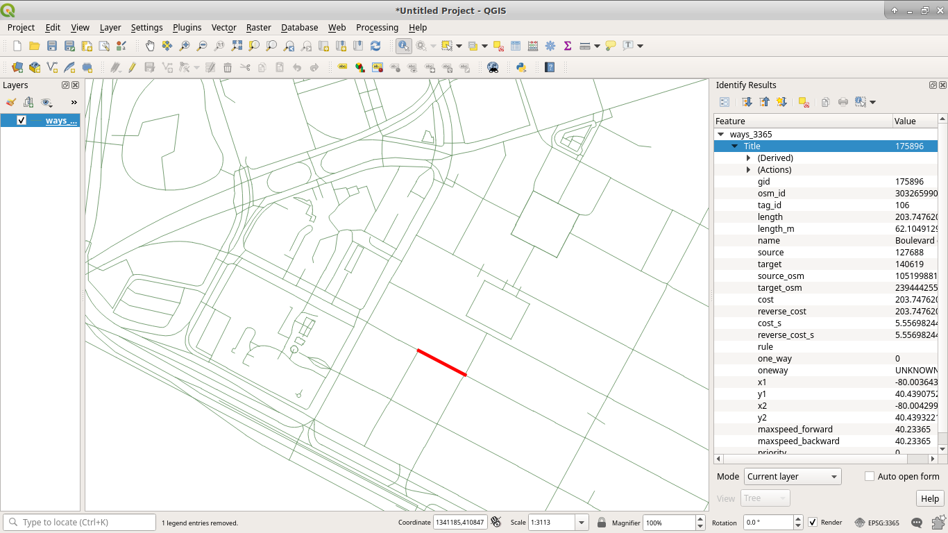
That same road is now "203.747620652544" which seems like a reasonable
number of feet. (It's also spot on the length_m (length in meters)
field, that is part of the OSM import, when converted to feet!)
Finding all roads within a certain distance of a stop
Now, a walkshed is how far you can walk on the road for a certain distance. To clarify why this is important, take the yellow bus stop below. The grey circle is ¼mi (1230ft) buffer around it. This buffer includes part of a loop of road to the south. However, the pale orange line of the ruler shows that you'd need to walk along 0.3mi of road to get to the point from our starting spot.
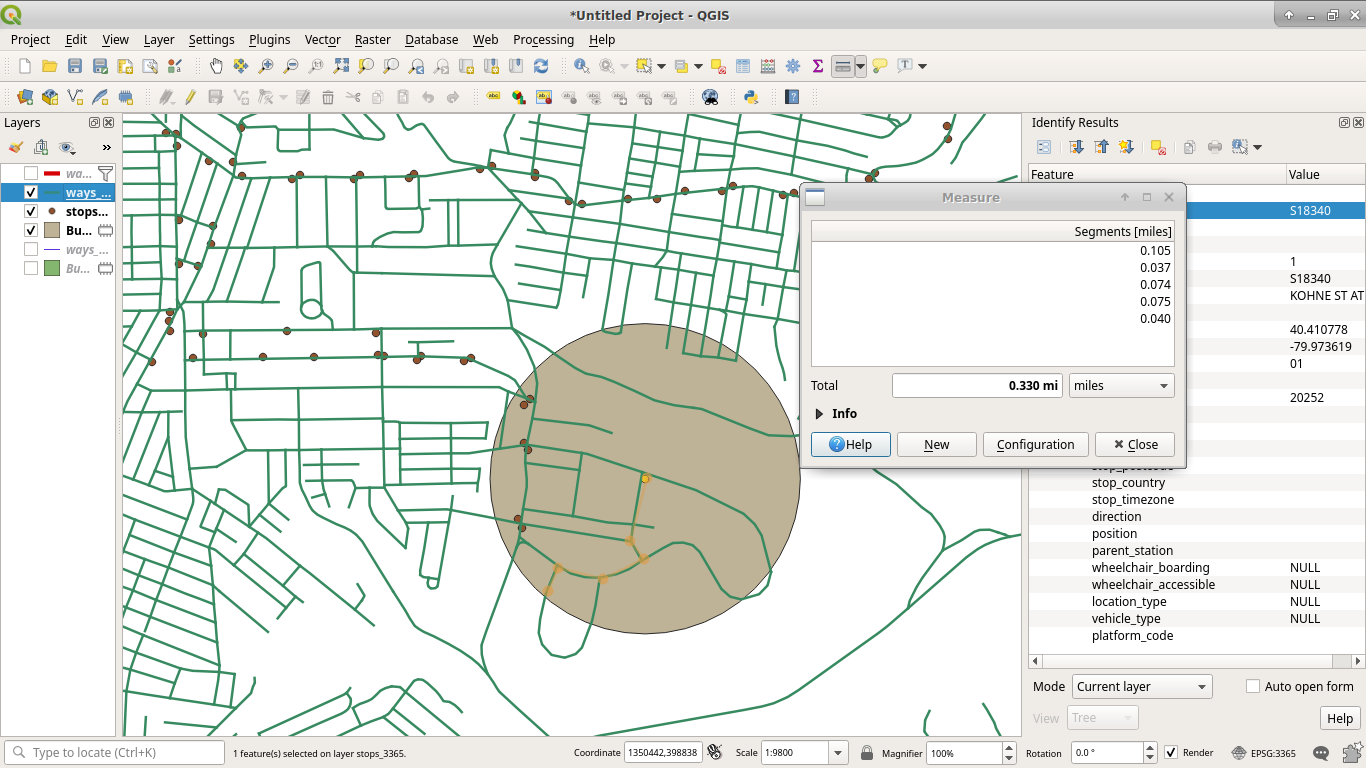
What we need is a function that takes the road network and provides the distance you'd walk or drive on the road from a starting point to get somewhere, since we can't just build a buffer around each point.
pgRouting provides a handy function that does exactly what we're looking
for:
pgr_drivingDistance.
We give pgr_drivingDistance a query containing our weighted graph as a
table of (edge id, source vertex id, target vertex id, cost, reverse
cost). We need to select reverse cost, otherwise pgr_drivingDistance
will be forced to traverse every road from start to end, and not end to
start, so we'd be at the mercy of how the road was imported. There are
ways to take "one-way" roads into account, but since we're dealing with
pedestrians, we'll ignore that.
We also give pgr_drivingDistance a source vertex id and a maximum
distance, and it returns every segment of road in the source graph, and
the aggregate cost to get there, that is within the distance given.
The following query computes the walkshed. I store it directly in a table because it takes north of 2 hours to run on my machine. I'm still working on making this faster, but since we're essentially computing it once and will reüse these results, it's not a huge problem in practice.
What's happening here is I build a
CTE that is the
result or running pgr_drivingDistance for each stop. Notice the
keyword lateral in the join. Lateral
Subqueries
allow the execution of the subquery for each record in the FROM
clause; otherwise the subquery is executed independently of the rest of
the query.
I then build a CTE that pulls in all road segments that have a start or
end point that is the source or target from our results. I do this,
instead of just going by the edges returned fro pgr_drivingDistance
because if a particularly long segment or road (which isn't unheard of
if we were doing this for ¼mi) would not be included and it would
skew our results by not counting that area, even if it may be within our
walkshed. I'm erring on the side of including a few features further than
I want to avoid not including features I want.
Then, because of how the join was done, we simply group everything by
stop and road segment, pulling the smallest distance to a vertex for a
segment of road. (Remember, pgr_drivingDistance gives the distance a
vertex is from the start based on the edges in the graph.) However,
let's focus on a single stop, 'S18340', first since computing walksheds
for all stops takes a good while.
create table stops_walkshed_S18340 as
with all_within as (
  select stop_id, dd.*
  from gtfs.stops_3365
  join lateral (
    select seq, node, edge, cost, agg_cost
      from pgr_drivingDistance(
            -- We need to select reverse cost, otherwise
            -- pgr_drivingDistance will be forced to traverse every road
            -- from start to end, and not end to start, so we'd be at the
            -- mercy of how the road was imported. There are ways to take
            -- "one-way" roads into account, but since we're dealing with
            -- pedestrians, we'll ignore that.
            'SELECT gid as id, source, target, cost, reverse_cost ' ||
            'FROM osmpgrouting.ways_3365 ' ||
            -- Find all road segments that begin or end within the
            -- distance we're looking for. We're going to do 1mi to give
            -- ourselves some flexibility later on, and it doesn't
            -- substantually increase the walltime.
            'where st_dwithin(' ||
              -- This awkwardness is because pgRouting functions take
              -- text to run as a query to get the edges and vertecies,
              -- not the results of a subquery.
              'ST_GeomFromEWKB(decode(''' || stops_3365.the_geom::text  || ''', ''hex'')), ' ||
              'ST_StartPoint(ways_3365.the_geom), ' ||
              '5280) or' ||
            ' st_dwithin(' ||
              'ST_GeomFromEWKB(decode(''' || stops_3365.the_geom::text  || ''', ''hex'')), ' ||
              'ST_EndPoint(ways_3365.the_geom), ' ||
              '5280)',
        -- Start from the nearest vertex/intersection to the bus stop.
        (select id
          from osmpgrouting.ways_vertices_pgr_3365
          order by ways_vertices_pgr_3365.the_geom <-> stops_3365.the_geom
          limit 1),
        5280
    )
  ) dd
    on true
  where stop_id = 'S18340'
), simplified as (
  select
    gid, stop_id, agg_cost,
    the_geom
  from all_within
  join osmpgrouting.ways_3365
    on node in (source, target)
)
-- When we do the join above, a road segment could be pulled in
-- multiple times for a single stop, so we'll collect it and count
-- it as the min of either its start or end vertecies.
select gid, stop_id, min(agg_cost) as agg_cost, the_geom
from simplified
group by stop_id, gid, the_geom
;
We still have issues with portions of roads that have other portions outside the distance we're shooting for. To solve this, we're going to split each road into 100ft segments.
source and target are used by pgr_drivingDistance to connect
segments, so we need to ensure that they are still consistent. Examining
the data shows that the max edge and vertex ids are 6 digits longs.
census=# select max(gid) as max_gid, max(source) as max_source, max(target) as max_target from osmpgrouting.ways_3365;
 max_gid | max_source | max_target
---------+------------+------------
  287229 |     216247 |     216247
(1 row)
Additionally, gid is a bigint, which maxes out at 9223372036854775807,
which is 19 digits long. As such, I can create a new vertex id that is
the "packed" version of the old vertex id, the edge id, and the sequence
in the split. For example, if I had an edge with gid=287229 and a
source=216247, and it's the 4th segment after splitting, I can call
this new vertex 287229216247000004. Adding some special logic to keep
the original source and targets the same as they were in the
original data (but formatted appropriately), we can still use the
ways_vertices_pgr vertex table as well. (Note that I got a good
portion/idea for this query from the
ST_LineSubString
documentation.) (This does take a while to run.)
create table osmpgrouting.ways_3365_split100 as
select
    (to_char(gid, 'FM000000') || to_char(n, 'FM000000'))::bigint as gid
    osm_id,
    tag_id,
    st_length(new_geom) as length,
    name,
    cast(case
      when n = 0 then to_char(source, 'FM000000') || '000000000000'
      else to_char(source, 'FM000000') || to_char(gid, 'FM000000') || to_char(n, 'FM000000')
    end as bigint) as source,
    cast(case
      when end_percent = 1 then to_char(target, '000000') || '000000000000'
      else to_char(source, 'FM000000') || to_char(gid, 'FM000000') || to_char(n+1, 'FM000000')
    end as bigint) as target,
    st_length(new_geom) as cost,
    st_length(new_geom) as reverse_cost,
    new_geom as the_geom
from (select *, greatest(length,1) as orig_length from osmpgrouting.ways_3365) as x
cross join generate_series(0,10000) as n
join lateral (
      select 100.00*n/orig_length as start_percent,
      case
       when 100.00*(n+1) < orig_length then 100.00*(n+1)/orig_length
       else 1
      end as end_percent
)y on n*100.00/orig_length< 1
join lateral (
    select st_linesubstring(the_geom, start_percent, end_percent) as new_geom
)z on true
;
-- Some lines end up as a single point. Something to look into more :/
delete from osmpgrouting.ways_3365_split100 where ST_GeometryType(the_geom) = 'ST_Point';
alter table osmpgrouting.ways_3365_split100 add primary key (gid);
alter table osmpgrouting.ways_3365_split100 owner to census;
alter table osmpgrouting.ways_3365_split100 alter column the_geom type geometry(linestring, 3365) using st_setsrid(the_geom, 3365);
create index ways_3365_split100_the_geom_idx on osmpgrouting.ways_3365_split100 using gist(the_geom);
create index ways_3365_split100_source_idx on osmpgrouting.ways_3365_split100(source);
create index ways_3365_split100_target_idx on osmpgrouting.ways_3365_split100(target);
vacuum full osmpgrouting.ways_3365_split100;

create table osmpgrouting.ways_vertices_pgr_3365_split100 as select * from osmpgrouting.ways_vertices_pgr_3365;
update osmpgrouting.ways_vertices_pgr_3365_split100 set id = (to_char(id, 'FM000000') || '000000000000')::bigint;
create index ways_vertices_pgr_3365_split100_the_geom_idx on osmpgrouting.ways_vertices_pgr_3365_split100 using gist(the_geom);
vacuum full osmpgrouting.ways_vertices_pgr_3365_split100;
Now, we can run our walkshed calculation again. However, we can clean it up a little as well, now that we have much smaller segments to work with. Again, just for S18340 because we want to iterate quickly.
create table stops_walkshed_s18340_split100 as
with all_within as (
  select stop_id, dd.*
  from gtfs.stops_3365
  join lateral (
    select seq, node, edge, cost, agg_cost
      from pgr_drivingDistance(
            'SELECT gid as id, source, target, cost, reverse_cost ' ||
            'FROM osmpgrouting.ways_3365_split100 ' ||
            'where st_dwithin(' ||
              'ST_GeomFromEWKB(decode(''' || stops_3365.the_geom::text  || ''', ''hex'')), ' ||
              'ways_3365_split100.the_geom, ' ||
              '5280)',
        (select id
          from osmpgrouting.ways_vertices_pgr_3365_split100
          order by ways_vertices_pgr_3365_split100.the_geom <-> stops_3365.the_geom
          limit 1),
        5280
    )
  ) dd
    on true
  where stop_id = 'S18340'
), all_within_simplified as (
  select stop_id, node, max(agg_cost) as agg_cost
  from all_within
  group by stop_id, node
)
select
  gid, stop_id, agg_cost, the_geom
from all_within_simplified
join osmpgrouting.ways_3365_split100
  on node in (source, target);
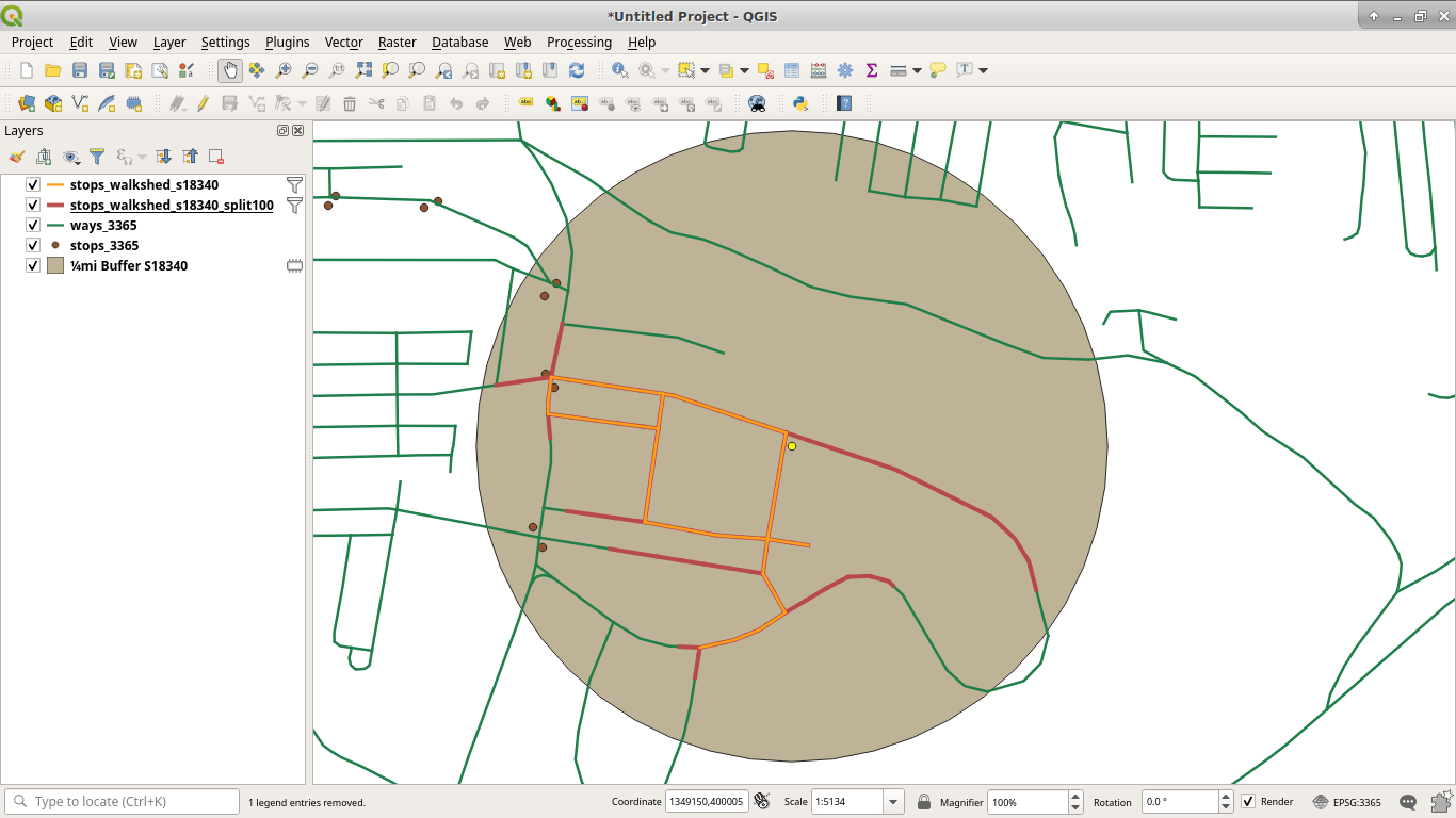
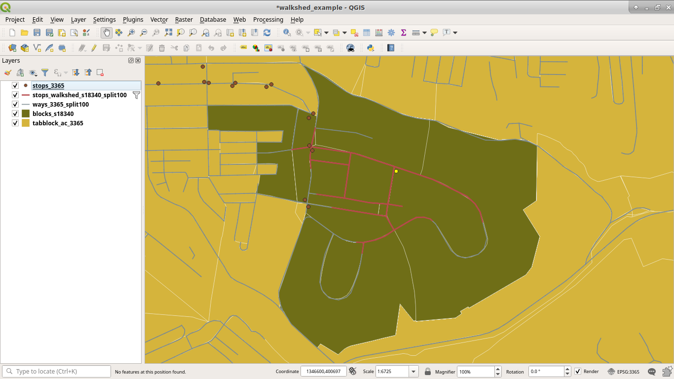
Below is a much more accurate representation of the walkshed in red, which was computed after splitting the road into segments. The orange was the "¼ mi" walkshed before we split the road into segments, and it misses a good portion of territory.
Since we computed the walkshed out to 1mi, and we stored the aggregate distance for each segment, we can use that to build heat maps of what's within a certain distance of a stop.

Let's now join the walkshed against our block data. Since the road features themselves might not overlap a block, since we're using different data sources, it's highly likely that a road might be on one side or the other of the block boundary. What we can do is build an arbitrary buffer along the road segment, i.e. make it "thicker", and test if the buffer overlaps a block. I chose 10ft. I also chose to filter only for blocks within ¼mi, and not build the distance metrics into the block.
create table blocks_s18340 as
select b.*
from tiger2017.tabblock_ac_3365 b
join stops_walkshed_s18340_split100 ws
  on st_overlaps(b.geom, st_buffer(ws.the_geom, 10))
where ws.agg_cost <= 1230;
The blocks themselves are delineated by a road or one of the white lines. Each block that was adjacent to one of the red lines is now selected in dark yellow. (As opposed to the rest of the blocks in a lighter yellow, mustard if you will.) This does add a bit to what the "walkshed" technically is, but at this point I'm not willing to interpolate population by building an arbitrary buffer over the walkshed, as when blocks are large it's likely that the population is not evenly spread among it and interpolation can give rather odd results. (See Interpolating Old Census Data for some discussion of those issues.) Using adjacent blocks is more than sufficient for our purposes, and at worst will overestimate slightly.
Now, let's remove the where stop_id = 'S18340' and compute the
walkshed and adjacent blocks for each stop!
create table stops_walkshed_5280 as
with all_within as (
  select stop_id, dd.*
  from gtfs.stops_3365
  join lateral (
    select seq, node, edge, cost, agg_cost
      from pgr_drivingDistance(
            'SELECT gid as id, source, target, cost, reverse_cost ' ||
            'FROM osmpgrouting.ways_3365_split100 ' ||
            'where st_dwithin(' ||
              'ST_GeomFromEWKB(decode(''' || stops_3365.the_geom::text  || ''', ''hex'')), ' ||
              'ways_3365_split100.the_geom, ' ||
              '5280)',
        (select id
          from osmpgrouting.ways_vertices_pgr_3365_split100
          order by ways_vertices_pgr_3365_split100.the_geom <-> stops_3365.the_geom
          limit 1),
        5280
    )
  ) dd
    on true
), all_within_simplified as (
  select stop_id, node, max(agg_cost) as agg_cost
  from all_within
  group by stop_id, node
)
select
  gid, stop_id, agg_cost, the_geom
from all_within_simplified
join osmpgrouting.ways_3365_split100
  on node in (source, target);
delete from stops_walkshed_5280 where ST_GeometryType(the_geom) = 'ST_Point';
vacuum full stops_walkshed_5280;
alter table stops_walkshed_5280 alter column the_geom type geometry(linestring, 3365) using st_setsrid(the_geom, 3365);
create index stops_walkshed_the_geom_idx on stops_walkshed using gist (the_geom);


create table stop_walkshed_blocks as
with stop_walkshed_buffer as (
  select stop_id, st_buffer(st_collect(the_geom), 10) as geom
  from stops_walkshed ws
  where ws.agg_cost <= 1230
  group by stop_id
)
select  b.gid, b.geoid10, stop_id, b.geom
from stop_walkshed_buffer swb
join tiger2017.tabblock_ac_3365 b
  on st_overlaps(b.geom, swb.geom);
(The reason I used a CTE is because I wantd to limit the number of blocks joined against. I didn't exhustively test performance against the more naïve query of
create table stop_walkshed_blocks_2 as
  select b.gid, b.geoid10, stop_id, b.geom
  from tiger2017.tabblock_ac_3365 b
  join stops_walkshed_5280 ws
    on st_overlaps(b.geom, st_buffer(ws.the_geom, 10))
  where ws.agg_cost <= 1230;
as the CTE version ran fast enough and I was running out of time alloted for this step.)
And Voilà, we have our walkshed.
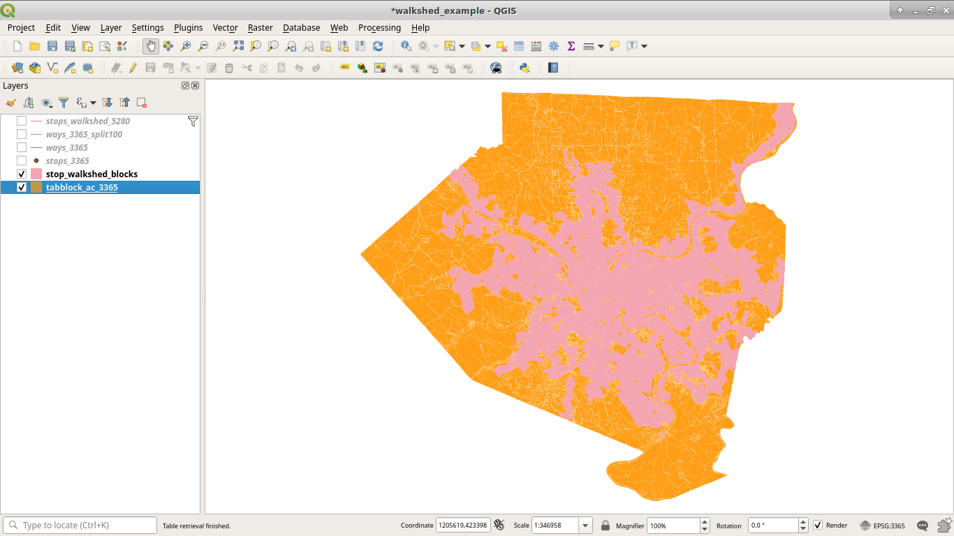
Now, to calculate the area of the county served.
select
(select sum(st_area(geom)) from (select geom from stop_walkshed_blocks group by geom)x)
/
(select sum(st_area(geom)) from tiger2017.tabblock_ac_3365);
Which yields just over 34% of the county by area.
In the next part, we'll import the cenus records and compute the percent of the population served. While that seems low, I expect the percent of population to be substantially higher, as the parts of the county not covered in pink have a much lower density (and in some cases are very much rural).