About Me!

This blog is about my musings and thoughts. I hope you find it useful, at most, and entertaining, at least.
Other Pages
Presence Elsewhere
Analyzing Bus Routes to Find Transit Deserts
Date: 2014-09-11
Tags: transit transportation Pittsburgh PAT Allegheny_County GIS topology QGIS GRASS PostGIS
I have recently become involved with Pittsburghers for Public Transit where I’ve volunteered to help make maps and do spatial and socio-economic analysis to help them better understand the problems areas face. One of the first things I did, part as a demo and part to help provide a little more information for their Baldwin campaign. I will cover importing and using Census data and importing it and TIGER data in a later entry; here I want to focus on topographic analysis done with part of the TIGER data and PAT’s GTFS data to identify area that are further than a given threshold from a public transit stop.
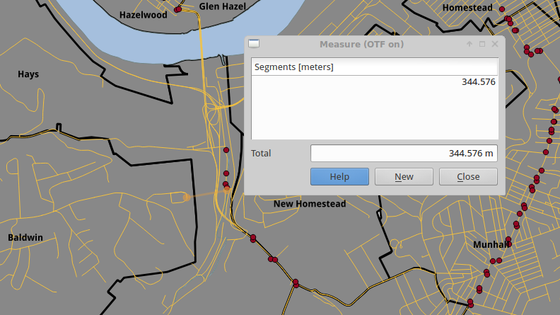
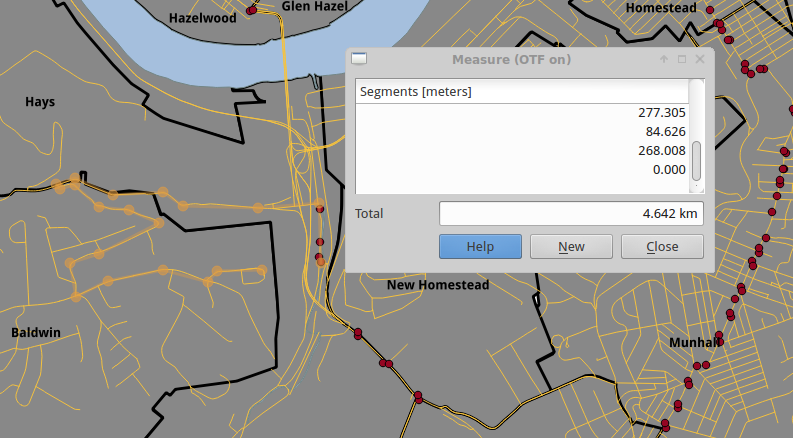
The first method I tried was to simply draw buffers, everything within a radius of a point, around each bus stop. Since buffers don’t consider anything but way-the-crow-flies (geodesic) distance they included parts of communities that can’t be accessed in anywhere near that distance. Take the following two maps (roads in orange, busstops as red dots); the first shows the geodesic distance from the closest busstop to a road. The second shows the shorted on-the-road (topographic) distance to it. An additional point, the space between the between the road and the busstop is not walkable (too steep), moreover, people should not have to walk through muck to get to their bus.
What I needed was a way to do Topographic or Network instead of straight geodetic analysis. I found that GRASS GIS is capable of doing the analysis I needed, and decided to give it a shot. I followed a tutorial, Basic Network Analysis With GRASS that was very close to what I wanted to be able to do. However, I kept getting nonsensical answers.
I eventually realized that my road map had very large segments for each road. In essence, the algorithm would think that the road it was on was very long, and all of the roads connected to it were too, so none of them were under the length limits I was looking for. To fix this issue, I split all of the roads into smaller parts. How I did this, and then how the analysis was performed is as follows.
I’m working on an Ubuntu 14.04 box, but the commands should be similar for most Unix-like OSs. I assume that PostgreSQL and PostGIS are installed.
Backstory
TIGER data is projected in EPSG 4269 (for some explanation as to why, see this comment on StackOverflow. This projection measures distance in units of arc, which isn’t the most intuitive unit to work in for the type of analysis we want to do (Is walking 13-arcseconds (0.0036 degrees) a short distance? (It’s a quarter mile on the equator)). In order to just ignore all of that, I decided to use the EPSG 2272 (Pennsylvania South (ftUS)) project.
This is known as a “State Plane” and is used by most state agencies in the southern part of Pennsylvania (where Allegheny County is). The project is in feet, therefore distances can be measured in a straight-forward manner.
Creat the database
createdb topotest
echo "CREATE EXTENSION postgis;" | psql topotest
Data Gathering
First let’s grab the TIGER road map for Allegheny County (FIPS code 42003 (42 is Pennsylvania, 003 is the county in the state.)) (Fun fact, FIPS codes are in alphabetical order and often skip codes so that new ones may be added without having to lose that order or re-arrange them).
mkdir geodata
cd geodata
wget ftp://ftp2.census.gov/geo/tiger/TIGER2014/ROADS/tl_2014_42003_roads.zip
mkdir tl_2014_42003_roads
unzip -d tl_2014_42003_roads tl_2014_42003_roads.zip
shp2pgsql -s 4269:2272 -W LATIN1 -I tl_2014_42003_roads.shp > tl_2014_42003_roads.sql
cat tl_2014_42003_roads.sql | psql topotest
For shp2pgsql, the -s 4269:2272 tells it to convert from the input SRID to the output SRID (in this case the NAD-83 projection to Pennsylvania-South). -W LATIN1 defines the encoding that the text in the shapefile’s database is in, and -I tells it to create spatial indices.
Once imported, cd .. to get back to the geodata directory.
Download the zip from the Port Authority (click “Download Port Authority GTFS files “).
mkdir pat_gtfs
unzip -d ~/geodata/pat_gtfs ~/Downloads/general_transit_CleverTripID_1409.zip
To import this data into our database, we’re going to use my fork of gtfs_SQL_importer originally from cbick as his appears abandoned and some bugs needed fixed for newer versions of PostGIS. This, boys and girls, is one of the main reasons Free Software is great!
git clone https://github.com/jimktrains/gtfs_SQL_importer.git
cd gtfs_SQL_importer/srccat gtfs_tables.sql | psql topotest
python import_gtfs_to_sql.py ~/geodata/pat_gtfs | psql topotestcat gtfs_tables_makespatial.sql | psql topotest
cat gtfs_tables_makeindexes.sql | psql topotest
cat vacuumer.sql | psql topotest
Cleanup the data
Use psql topotest to login to your database and get a shell.
ALTER TABLE gtfs_stops ALTER COLUMN the_geom TYPE Geometry(Point, 2272) USING ST_Transform(the_geom, 2272);ALTER TABLE gtfs_shape_geoms ALTER COLUMN the_geom TYPE Geometry(LineString, 2272) USING ST_Transform(the_geom, 2272);
Now to break apart the road segments into smaller segments; what the following query does is read each pair of successive segments and creates records with only that simple line and the reset of the road’s metadata.
CREATE TABLE roads AS ( SELECT gid, linearid, fullname, rttyp, mtfcc, geom, ST_Length(geom) as length FROM ( SELECT gid, linearid, fullname, rttyp, mtfcc, ST_MakeLine(sp, ep) AS geom FROM ( SELECT gid, linearid, fullname, rttyp, mtfcc, ST_PointN(geom, generate_series(1, ST_NPoints(geom)-1)) as sp, ST_PointN(geom, generate_series(2, ST_NPoints(geom) )) as ep FROM ( SELECT gid, linearid, fullname, rttyp, mtfcc, (ST_Dump(geom)).geom AS geom FROM tl_2014_42003_roads ) AS lines ) AS segments ) AS mostly_there
);CREATE INDEX roads_geom_idx ON roads USING GIST (geom);
CREATE INDEX roads_gid_idx ON roads (gid);
CREATE INDEX roads_linearid_idx ON roads (linearid);
ALTER TABLE roads ADD COLUMN id BIGSERIAL NOT NULL PRIMARY KEY;SELECT UpdateGeometrySRID(‘roads’, ‘geom’, 2272);
Network analysis with GRASS
GRASS can be controlled fully via a command line or via the menus. If you’re new to GRASS, I would suggesst hunting around in the menus to see what features it offers. In a very helpful gesture, each menu option provides the name of the command it’s an interface to.
First, we’ll import the vector data (File > Import Vector Data > Common Input Formats [v.in.ogr]) GRASS can connect directly to PostgreSQL databases, which makes it very easy to import the data already in our database.
v.in.ogr dsn=PG:dbname=topotest layer=roads output=roads
v.in.ogr dsn=PG:dbname=topotest layer=gtfs_stops output=stops
Once loaded, the busstop layer needs to be connected to the road, otherwise you can’t get to them via the road! (Vector > Network analysis > Network maintenence [v.net])
v.net input=roads points=stops output=network operation=connect thresh=100
Additionally, lets add the stop metadata as part of the network. (Database > Vector database connections > Set vector map – database connection [v.db.connect])
v.db.connect map=network table=stops layer=2
Now for the guts of the analysis. We need to categorize all of the roads according to how far away the nearest busstop is. These are called isolines. (Vector > Network analysis > Split net [v.net.iso])
v.net.iso --overwrite input=network output=network_isolines ccats=1-10 costs=1320,2640,3960,5280,6600,7920,9240,10560 afcolumn=LENGTH abcolumn=LENGTH
The astute reader would notice two things:
- Our cost thresholds are quarter-mile increments
- There are almost 7000 busstops (categories) that were loaded, and that we’re now using 10?
The reason we’re only using 10 busstops is because running the entire network takes roughly 6.5hrs on my laptop. For testing purposes, the more-or-less instant gratification that 10 stops will provide suffices.
Visualization
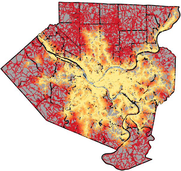
If we assign the iso-lines random colors with d.vect -c network_isolines, we can get a quick glimpse of the output. (In quarter mile increments: grey, light red, dark red, green, dark green, blue, yellow, dark yellow).
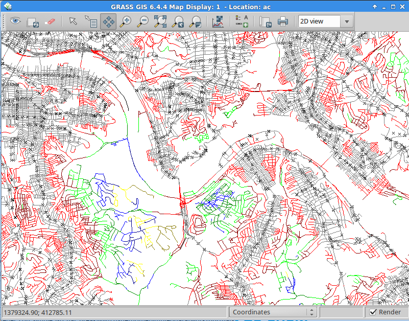
As you can see, the little area we were looking at above is dark-yellow, indicating that it is in the > 2mi isoline. Now, this isn’t a very pretty visualization. Let’s export it to a shapefile and load it into QGIS. Once loaded, we’ll categorize the layer with the `cat` field and use a color ramp to show differences in distance.
Zooming in we can look at the area we’ve been focusing on.
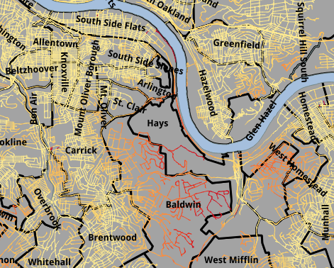
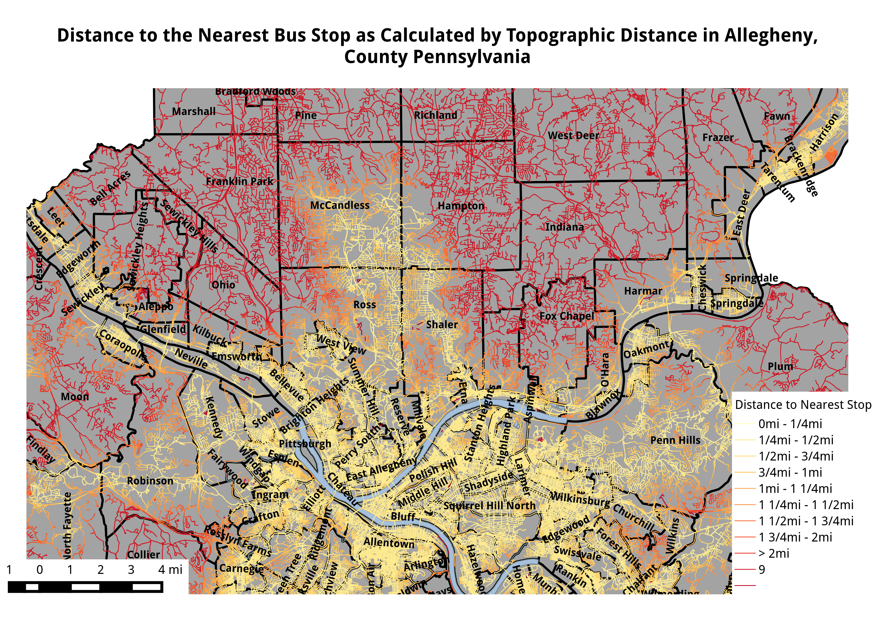
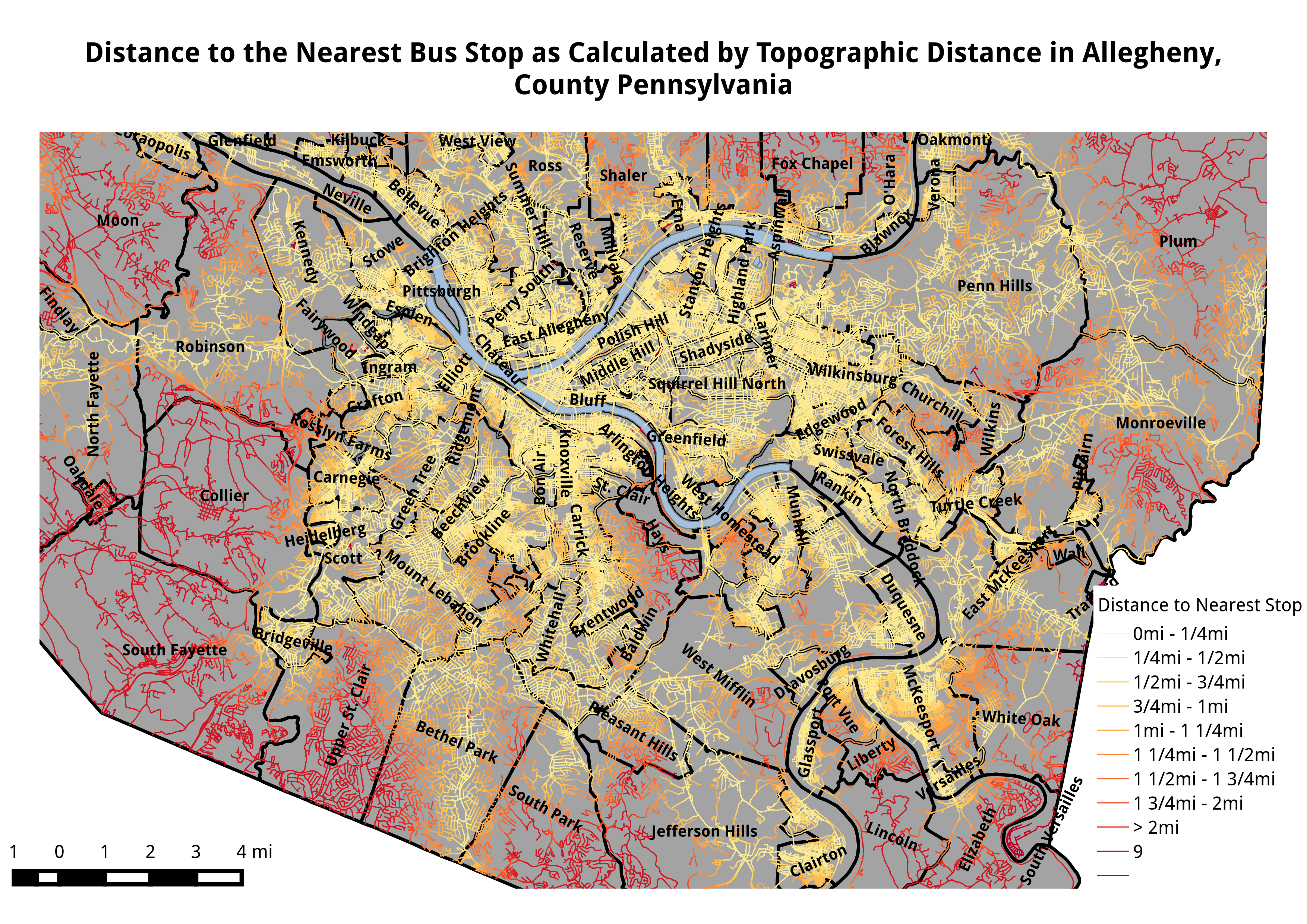
Zooming out we can look at the entire county.
It’s plain to see that the transit network covers only the most densely populated area, visually identifiable by a high concentration of roads. However, it does not service all of these area. Further comparison with Census data would yield better results.
Slightly more zoomed in, but very large, images can be found here: North part of the County and South part of the County
Future
There are many things I would like to do with this data, but one of the firsts would be to incorporate DEM into the model so-as to take grades (which we have a lot of over in Pittsburgh) into the cost calculation.
Also, I need to ensure that bridges don’t become intersections, as that introduces a source of error into the calculations.
Another piece of information is to use the GTFS data we’ve already loaded to come up with frequencies. That would enable us to look for areas that are, for instances, not within walking distance of a bus that comes less frequently than every half-an-hour.